The Simplest Algorithm You Can Think About: KNN

Passionate about leveraging AI, big data, and computer vision to extract meaningful insights and drive technological advancements. With a strong foundation in data science, I specialize in satellite image analysis, deep learning, and predictive modeling to solve complex real-world challenges.
Introduction
When people hear machine learning, they often imagine massive neural networks powering self-driving cars or chatbots like ChatGPT. But the journey doesn’t start with deep learning — it starts with something much simpler.
In fact, one of the first algorithms you’ll meet in machine learning is so intuitive that you’ve probably used it in real life without knowing: the K-Nearest Neighbors (KNN) algorithm.
This article is part of my SIMPLE ML series, where I explain ML concepts in the simplest way possible — the way I’m learning them myself. Today, we’ll see how KNN works, why it’s easy to understand, and what kind of results you can expect when you use it for image classification

The Intuition:
Think of classification like sorting fruits. You already know what apples and oranges look like. Now you see a new fruit — it’s green, and you’re not sure if it’s an apple or an orange.
Instead of guessing, you look at the fruits closest to it:
If we choose k=3, we check the 3 nearest fruits.
Suppose the nearest fruits are 2 apples and 1 orange.
Since the majority are apples, we classify the green fruit as an apple.
This is the heart of the K-Nearest Neighbors (KNN) algorithm:
“To classify something new, look at its closest examples and let them vote.”
It’s incredibly simple — no equations yet, just common sense: objects are likely to belong to the same category as their closest neighbors.

Mathematical Definition:

The KNN algorithm works as follows:
Compute distances
For each training example xix_ixi, calculate its distance from the new fruit x.
Common choices:


Find k nearest neighbors
- Pick the K training examples with the smallest distances.
Majority voting
- The predicted label is the one that appears most among those K neighbors:

Example (Fruit Case with K=3)
Compute the distance from the green fruit to all apples and oranges.
Find the 3 closest fruits.
If 2 are apples and 1 is an orange → predict an apple.
Choosing Hyperparameters
Unlike some ML models that learn parameters automatically, KNN relies on a couple of choices we need to make ourselves — these are called hyperparameters.
The value of K:
If K = 1: The prediction is simply the label of the closest neighbor.
- (Very sensitive to noise (one mislabeled point can cause errors).
If K is larger (e.g., 3, 5, 7), predictions become more stable because we take a majority vote among multiple neighbors.
If K is too large, the model becomes too “smooth” and can ignore important local differences.

Rule of thumb:
Small K → more flexible, but noisy.
Larger K → smoother, but less sensitive to fine details.
Distance Metric:
L1 (Manhattan distance): works well when features are independent and sparse.
L2 (Euclidean distance): more common, gives smoother decision boundaries.
Other options: cosine similarity (often used in text & embeddings).
How to Choose Properly:
Never tune hyperparameters on the test set.
Use a validation set or cross-validation.
Try different values of K and different distance metrics. Pick the one that performs best on validation data

Real Dataset Demo:
Theory is nice, but machine learning only makes sense when we see it in practice. Let’s try KNN on two classic datasets.
Iris Dataset:
The Iris dataset has 150 examples of flowers, each described by 4 features (sepal length, sepal width, petal length, petal width). The goal is to classify flowers into Setosa, Versicolor, or Virginica.
Code (Python with scikit-learn):
  from sklearn.datasets import load_iris
  from sklearn.model_selection import train_test_split
  from sklearn.neighbors import KNeighborsClassifier
  from sklearn.metrics import accuracy_score

  # Load dataset
  iris = load_iris()
  X, y = iris.data, iris.target

  # Split into train/test
  X_train, X_test, y_train, y_test = train_test_split(X, y, test_size=0.2, random_state=42)

  # Train KNN
  knn = KNeighborsClassifier(n_neighbors=3)
  knn.fit(X_train, y_train)

  # Test
  y_pred = knn.predict(X_test)
  print("Accuracy:", accuracy_score(y_test, y_pred))
Typical result: around 95–97% accuracy with K = 3.
Why use this dataset?
Easy to understand (flowers 🌸).
Small enough to run instantly.
Great for making 2D scatter plots (petal length vs petal width).


MNIST Handwritten Digits:
The MNIST dataset contains 70,000 grayscale images of handwritten digits (0–9). Each image is 28x28 pixels.

Code (Python with scikit-learn):
from sklearn.datasets import fetch_openml
from sklearn.model_selection import train_test_split
from sklearn.neighbors import KNeighborsClassifier
from sklearn.metrics import accuracy_score

# Load MNIST (this may take a while the first time)
mnist = fetch_openml('mnist_784', version=1)
X, y = mnist.data, mnist.target.astype('int')

# Train/test split
X_train, X_test, y_train, y_test = train_test_split(X, y, test_size=0.1, random_state=42)

# Use smaller subset for speed
X_train_small, y_train_small = X_train[:5000], y_train[:5000]
X_test_small, y_test_small = X_test[:1000], y_test[:1000]

# Train KNN
knn = KNeighborsClassifier(n_neighbors=3)
knn.fit(X_train_small, y_train_small)

# Test
y_pred = knn.predict(X_test_small)
print("Accuracy:", accuracy_score(y_test_small, y_pred))
Typical result:
K=1 → ~95% accuracy
K=3 or 5 → ~96–97% accuracy
But prediction is very slow because each test digit compares to thousands of training digits.
Why use this dataset?
It’s the “Hello World” of image classification.
Readers instantly recognize digits.
Shows the limits of KNN → too slow for large datasets.
Results & What to Expect
Running KNN yields two main types of results: numerical (accuracy) and visual (plots/confusion matrices). Let’s see what they mean.
Accuracy vs k:
When we vary the number of neighbors kkk, accuracy changes:
| Dataset | k=1 | k=3 | k=5 | k=7 | k=9 |
| Iris 🌸 | ~94% | ~96% | ~96% | ~95% | ~94% |
| MNIST 🔢 | ~95% | ~96% | ~97% | ~96% | ~95% |

Insights:
K = 1 is often noisy.
K = 3 or 5 usually gives the best balance.
Too large K → accuracy starts to drop.
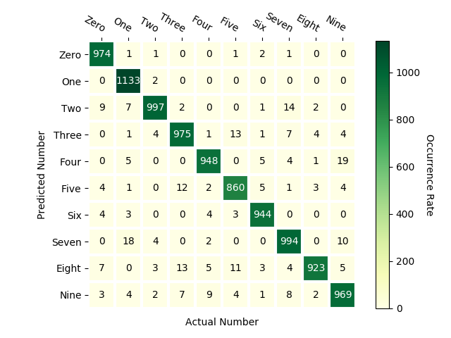
Confusion Matrix:
For multi-class datasets like MNIST (digits 0–9), accuracy alone doesn’t tell the full story. A confusion matrix shows which classes are being confused:
Diagonal = correct predictions.
Off-diagonal = mistakes.
Example:
4 is often misclassified as 9.
5 is sometimes mistaken for 6.

Speed & Practical Limits:
Training: almost instant (KNN just stores the data).
Prediction: very slow, because each new test image is compared with every training image.
Example: Classifying 1,000 test digits with 5,000 training digits → 5 million comparisons.
This is why KNN is primarily a teaching tool, rather than a production model for image classification.
Takeaway:
KNN can reach ~97% accuracy on MNIST with the right k.
It’s surprisingly strong for small, low-dimensional datasets.
But for large, high-dimensional data like images, it becomes slow and inaccurate compared to modern models.
Loss Function & Evaluation
Unlike neural networks or linear regression, the KNN algorithm doesn’t minimize a loss function during training. Why? Because there’s no “training” in the usual sense — the model just stores the data.
But once we start making predictions, we need a way to measure performance. That’s where evaluation metrics come in.
Classification Error:
The simplest measure is the error rate:
\text{Error Rate} = \frac{\text{# of wrong predictions}}{\text{total predictions}}
Or equivalently, accuracy:

Example:
- If we test 100 images and KNN gets 92 correct → Accuracy = 92%, Error Rate = 8%.
Confusion Matrix
For multi-class problems (like MNIST digits 0–9), the error rate is not enough. A confusion matrix shows:
Which classes are correctly predicted (diagonal)?
Which classes are often confused with others (off-diagonal)?
Example: In MNIST, digit “4” is sometimes confused with “9”.
Other Metrics (Optional)
If the dataset is imbalanced (some classes have more examples than others), we may also use:
Precision: How many of the predicted positives are correct?
Recall: How many of the actual positives are detected?
F1-score: Balance between precision and recall.
But for simple balanced datasets (Iris, MNIST), accuracy is usually enough.
Strengths and Weaknesses of KNN
Like every algorithm, KNN has its pros and cons. Understanding them helps you know when to use it — and when to avoid it.
Strengths:
Simple & Intuitive
Easy to explain with real-world analogies (neighbors voting).
No complicated math during training.
No Training Needed
KNN just stores the dataset.
Useful when you want quick deployment without model fitting.
Flexible
Works for classification, regression, and even recommendation systems.
Choice of distance metric makes it adaptable to different problems.
Good for Small Datasets
- Performs surprisingly well when data is low-dimensional and small (e.g., Iris dataset).
Weaknesses:
Slow at Prediction
To classify one new point, KNN compares it to every training example.
With large datasets, prediction becomes painfully slow.
Poor Distance Metrics for Images
Pixel-based distances (L1, L2) don’t capture perceptual similarity.
Two images that look the same to humans might have very different pixel values.
Curse of Dimensionality
High-dimensional data (like 28x28 images = 784 features) requires exponentially more training points to cover the space.
KNN struggles as dimensionality grows.
Memory-Heavy
Must store the entire training dataset.
Not efficient for devices with limited memory.

Key Takeaway:
KNN is great as a learning tool to understand data-driven classification.
But for real-world large datasets (like images), we need faster, more powerful models like linear classifiers and neural networks.
Conclusion & Next Steps
The K-Nearest Neighbors (KNN) algorithm is often the first stop in a machine learning journey. It’s simple, intuitive, and shows how we can let data itself drive classification decisions instead of writing hard-coded rules.
What we learned today:
KNN classifies new points by looking at their closest neighbors and taking a majority vote.
Distance metrics (L1 vs L2) define what “closeness” means.
The hyperparameter kkk controls the balance between flexibility and stability.
On small datasets like Iris or MNIST, KNN can achieve good accuracy.
But in practice, KNN struggles with speed, memory, and high-dimensional data — making it more of a teaching tool than a production algorithm.
Why it matters:
KNN introduces fundamental ML ideas:
Using distance to compare examples.
The concept of validation sets for tuning hyperparameters.
Evaluating models with accuracy and confusion matrices.
Next in SIMPLE ML
KNN shows us the data-driven approach to classification. But wouldn’t it be nice to have a model that learns patterns during training, instead of memorizing all data?
That’s exactly where we’re headed next:
👉 Linear Classifiers — the first step toward models that generalize better, run faster, and scale to bigger problems.


