From Pixels to Predictions: Linear Regression in Computer Vision

Introduction:

• Linear regression is like drawing a straight line that best fits the data points. In computer vision, we can use this simple idea to predict things from images. Even though it is a fundamental model, it helps us understand how machines can “learn” patterns from pictures.

• It is straightforward to grasp. It serves as a good “first step” before moving on to larger models like neural networks. Think of it as the “baby step” in learning computer vision.

Background – What is Linear Regression?

Linear regression is one of the simplest ideas in machine learning. Imagine you have many points on a piece of paper, and you want to draw a straight line that passes as close as possible to all of them. That line is your “prediction tool.” Whenever you see a new point, you can look at its position and use the line to guess its value.

In math language, this line is written as:

Here, X represents the input (in vision, this could be pixel values or features from an image), w is the weight that indicates the importance of each input, and b is a bias that shifts the line up or down. The output y is our prediction — for example, it could be the brightness of a pixel or the age of a person from their photo.

The machine “learns” by adjusting the values of www and bbb until the line fits the data as well as possible. This fitting process is done by minimizing something called the loss function, which usually measures how far off our predictions are from the true answers. The smaller the loss, the better our line is doing.

How Linear Regression Connects to Computer Vision?

So far, linear regression sounds like a math exercise with dots and lines. But in computer vision, the “dots” are not random — they come from images. An image is made up of thousands, sometimes millions, of pixels. Each pixel is just a number, showing how bright or dark it is. If it is a color image, each pixel has three numbers, one for red, one for green, and one for blue.

Now imagine flattening an image into a long list of numbers. Instead of seeing a 28×28 grid of pixels, we see a line of 784 values (28 multiplied by 28). This list becomes our input X. The job of linear regression is then to take this input and learn the best weights w and bias b to predict something about the image. That “something” could be the overall brightness, the presence of an object, or even a person’s age if we are working with face data.

In other words, linear regression allows us to connect raw pixel values or simple features from images to a meaningful continuous output. It is not powerful enough to capture the full complexity of vision tasks, but it gives us the first bridge between pictures and predictions.

Example Applications of Linear Regression in Vision:

Linear regression might look too simple for modern computer vision, but it actually has some interesting uses, especially as a starting point. Let’s look at a few examples.

One application is predicting pixel intensity. Suppose we have the coordinates of a pixel in an image (its row and column). Using linear regression, we can try to predict how bright that pixel is. This might sound small, but it shows how the model learns patterns in image structures, like gradients or smooth surfaces.

We can also use linear regression for feature-based tasks. Instead of raw pixels, we extract simple features such as the average brightness, the size of an object’s bounding box, or the number of edges in an image. These features are then used as inputs to linear regression, which predicts things like blur level, object size, or distance.

These examples show us that while linear regression cannot solve advanced tasks like recognizing cats and dogs, it plays a very important role in teaching us how to connect image information to predictions in a clear and interpretable way.

Implementation – Linear Regression with Images

To see how linear regression works in computer vision, let us try a simple experiment. We will take a dataset of small images, flatten each image into a list of numbers, and then train a linear regression model to predict a value. For simplicity, we will use the MNIST dataset (handwritten digits, 28×28 grayscale images). Our task will be to predict the average brightness of the digit image.

This is not a real-world problem, but it shows clearly how linear regression can connect image pixels to an output value.

Here is the code:

import numpy as np
from sklearn.datasets import fetch_openml
from sklearn.model_selection import train_test_split

# Load MNIST dataset (70,000 images, each 28x28 pixels)
mnist = fetch_openml("mnist_784", version=1)
X = mnist.data / 255.0     # scale pixels between 0 and 1
y = X.mean(axis=1)         # target = average brightness of the image

# Train/test split
X_train, X_test, y_train, y_test = train_test_split(X, y, test_size=0.2, random_state=42)

# Linear regression: closed form solution
w = np.linalg.pinv(X_train) @ y_train   # weights
y_pred = X_test @ w                     # predictions

# Evaluate with Mean Squared Error
mse = np.mean((y_pred - y_test)**2)
print("Test MSE:", mse)

In this code, every image is turned into 784 numbers (28×28). Linear regression then learns a set of weights that map these 784 inputs to a single value: the brightness. Finally, we measure how good the model is with the mean squared error.

What Did the Model “Learn” on MNIST? (Weight Map):

After training linear regression on MNIST to predict average brightness, we can peek inside the model by reshaping the learned weights w back into image form. Remember that www has one weight per pixel (784 numbers for a 28×28 image). If we reshape w into a 28×28 grid, we get a heatmap that shows which pixels the model considers more important.

In this visualization, brighter pixels mean stronger weights, while darker pixels mean weaker ones. This grayscale style is easier to read because you don’t need to think about color meaning — it’s simply “bright = important.” By looking at this weight map, we can see how even a simple linear model begins to recognize patterns in the data.

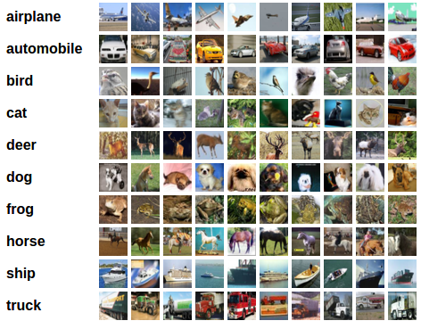
CIFAR-10 (Color Images) – Setup and a Simple Task:

CIFAR-10 is a small dataset of 60,000 color images, each 32×32 pixels with three color channels (red, green, blue). Unlike MNIST’s grayscale digits, CIFAR-10 includes varied objects (airplanes, cars, birds, cats, etc.), which makes learning harder.

To begin simply, we will use an easy continuous target: the average color of each image. For each image, we calculate three numbers—average red, average green, and average blue—and use linear regression to predict these three values from the raw pixels. This is a clear example of multi-output linear regression: the inputs are pixel values, and the outputs are three continuous color averages. Although it's not a "semantic" task, it demonstrates how a linear model can scale from one output (brightness) to multiple outputs (R, G, B) on a more complex dataset.

Now let’s try something more ambitious: predicting the class of a CIFAR-10 image using linear regression. Each CIFAR-10 image is 32×32×3 pixels, which equals 3,072 numbers when flattened. We give this long list to linear regression, and the model outputs 10 scores — one for each class. The class with the highest score becomes the prediction.

Here’s the code:

import numpy as np
from tensorflow.keras.datasets import cifar10
from sklearn.model_selection import train_test_split
from sklearn.metrics import accuracy_score

# Load CIFAR-10
(X_train_raw, y_train_cls), (X_test_raw, y_test_cls) = cifar10.load_data()
X = np.concatenate([X_train_raw, X_test_raw], axis=0).astype(np.float32) / 255.0
y_cls = np.concatenate([y_train_cls, y_test_cls], axis=0).reshape(-1)  # shape (60000,)

# One-hot targets (10 classes)
num_classes = 10
y_onehot = np.eye(num_classes)[y_cls]

# Flatten images
X_flat = X.reshape(len(X), -1)

# Train/test split
X_tr, X_te, Y_tr, Y_te, cls_tr, cls_te = train_test_split(
    X_flat, y_onehot, y_cls, test_size=0.2, random_state=42
)

# Closed-form regression: W is (features, 10)
W = np.linalg.pinv(X_tr) @ Y_tr

# Predict class scores
scores = X_te @ W
pred_cls = np.argmax(scores, axis=1)

# Accuracy
acc = accuracy_score(cls_te, pred_cls)
print("Linear regression accuracy:", acc)

This experiment usually gives low accuracy compared to models designed for classification, but it demonstrates how regression can be extended to multi-output tasks.

Linear Regression as a Classifier: Weaknesses

Even though we can stretch an image into a column of numbers and predict class scores, linear regression has serious limits in computer vision. The model does not know that neighboring pixels form edges, corners, or shapes. It sees the input only as a flat vector, losing all the 2D structure of the image.

This means the model struggles with changes in viewpoint, lighting, or cluttered backgrounds. It also uses a mean squared error loss against one-hot labels, which is not the right tool for classification. That’s why linear regression accuracy on CIFAR-10 is very low, and why we quickly move to better models such as logistic regression or convolutional neural networks (CNNs).

Why Linear Regression Struggles in Vision (Real-World Challenges)

Linear regression can handle simple tasks, but when it meets the real visual world, it breaks down. Let’s see this through our favorite example — cats.

Illumination: A cat in bright sunlight looks very different from a cat in shadow or at night. For us, they’re all cats, but for linear regression, the pixel values change so much that it sees them as different objects.

Viewpoint Variation: If you take a picture of a cat from the front, from the side, or from above, each image has completely different pixel arrangements. A linear model can’t connect these different views as being the same cat.

Deformation & Occlusion: Cats stretch, curl, or hide under blankets. Sometimes part of the cat is missing from view — maybe just the head or just the tail. Linear regression cannot cope with these flexible shapes or missing parts.

Background Clutter: A cat in an empty room is easy. But a cat in tall grass or in snow is much harder — the pixels from the background confuse the model. Linear regression has no way to focus on the cat and ignore the clutter.

These examples show why linear regression is not enough. It cannot generalize across lighting, angles, shapes, or backgrounds. This motivates us to move beyond linear regression to models that can truly understand the structure of images.

Conclusion & Next Steps:

We have taken our first steps in computer vision with linear regression. Starting from simple brightness prediction on MNIST, moving to color prediction in CIFAR-10, and even trying class scores, we saw how this basic model connects raw pixel values to meaningful outputs. Along the way, we visualized weight maps and discovered both the strengths and weaknesses of linear regression.

The key lesson is that while linear regression is simple and interpretable, it is not powerful enough for real-world vision. It cannot deal with changes in lighting, viewpoint, or clutter, and it ignores the spatial structure of images. Still, it gives us a foundation: the idea that learning means adjusting parameters (W and b) to reduce a loss and make better predictions.

And this is exactly where our journey continues. Before jumping into neural networks, we will pause to carefully study the core tools of learning:

• Loss functions – how we measure the difference between predictions and the truth.

• Optimization – the strategies for improving our model step by step.

• Gradient descent – the method that powers nearly all modern machine learning.

Once we understand these three pillars, we will be ready to move beyond linear regression into neural networks, where models learn not just straight lines but deep, flexible functions that can truly “see” patterns in images.